A short R tutorial

GGIR for those without prior R experience

R package GGIR has been designed with the ambition to be user-friendly without prior R experience. For example, usage of GGIR entails only a single function call that takes care of data loading, analyses, and report generation. The primary learning curve for new GGIR users is to become familiar with all the optional input arguments.

Nonetheless, for those without prior R experience it can be a challenge to find your way around the R environment itself. To help you with this, we have compiled the following R tutorial tailored to what we think you need to know about R in order to get started with GGIR.

1. R and RStudio
    1. Install R and RStudio, these are two separate pieces of software which complement each other.
    2. Open RStudio.


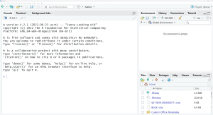
  1. If you already had R installed: Check which R version you are using, which is shown when you open RStudio at the top of the window named Console. Next, go to the R release history and verify that you are using an R version that is no more than 1 year old.
  2. If you already had RStudio installed: Check that it is up to date by clicking on the Toolbar: Help -> Check for updates.
2. Using an R script
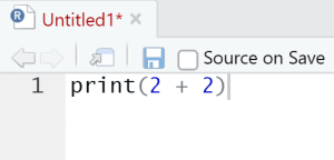
  1. Go to the RStudio Toolbar -> File -> New file -> script. This will open a new empty script.
  2. Type inside the script: print(2 + 2)
  3. The text print(2 + 2) is called R code.
  4. Save the file somewhere on your computer with Toolbar -> File -> Save as…
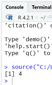
  5. Press the Source button in the top corner of your script.
  6. Do you see a 4 in the RStudio console window?
  7. Now put a hashtag in front of print(2 + 2) as in # print(2 + 2)
  8. Repeat steps 4 and 5.
  9. If all went well you do NOT see a 4 this time.
  10. This is because adding a # at the beginning of line comments out that line, which means that RStudio will not execute it.
  11. If you put the # at the END of a line of code then everything you type on the line after the # will be a comment. For example:
  12. Note that in other R introduction courses you may learn to type the R commands directly in the console window. We are not doing this because our GGIR commands are going to be long and it would be impractical to type them in the console. Instead we strongly recommend you to follow the steps above and work with R scripts for everything you do with GGIR.
3. Characters and vectors
  1. Replace the code by: print(“hello world”)
  2. Save the script (Hint on with Ctrl + S or Command + S on Mac is a short key to save a file without having to use the toolbar).
  3. Press again the Source button.
  4. Do you now see “hello world” in the RStudio console window?
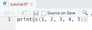
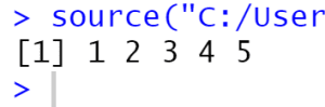
  5. Replace the code by: print(c(1, 2, 3, 4, 5))
  6. Save the script and press again the Source button.
  7. Do you now see 1 2 3 4 5 in the RStudio console window?
  8. What c() does is that it creates a vector from the character or numbers inside it.
  9. Replace the code by: print(1:5)
  10. Save the script and press again the Source button.
  11. Do you now see 1 2 3 4 5 again? This is correct, 1:5 is the same as c(1, 2, 3, 4, 5).
4. Using functions and looking up documentation
  1. Replace the code by: print(cor(x = 1:10, y = 2:11))
  2. Do you see a 1?
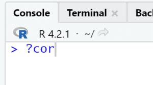
  3. You just used the R function cor. To look up what cor does, go to the console and type ?cor and press Enter.
  4. Do you now see the documentation for the cor function and can you tell what function cor calculates?
  5. As you may have noticed we are specifying an x and a y in the cor command. x and y are what we call function arguments to the function ‘cor’ and in this case the argument value specified for x is 1:10 and the argument value given for y is 2:11. In GGIR you will be working with a lot of function arguments which can have character values such as “hello world”, numeric values like 4, or numeric vector values such as c(1, 2, 3, 4, 5) or 1:5. Additionally we will be working with Boolean argument values, which can be TRUE or FALSE. Note that these have no quotes around them. For example, we will use Booleans to tell GGIR to do something or to not do something.
5. Specifying a file path
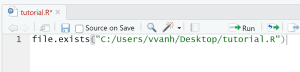
  1. Replace the code by file.exists(“C:/Users/vvanh/Desktop/tutorial.R”)
  2. Now edit this line such that it specifies a file that exists on your computer, it can be any file and does not have to be the tutorial.R file in this example.
  3. Save the script and press again the Source button.
  4. Do you now see TRUE in the console? If yes, then this means you specified the file path correctly. If you see FALSE then something went wrong. Keep trying until you see TRUE. Hint: R expects forward slashes, and when specifying a file always include the file extension (.xlsx, .txt, .docx, .bin, .gt3x, .cwa, .R, .csv, etcetera) even if your Windows file browser does not display them.
6. Specifying a folder path
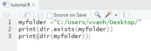
  1. Replace the code by myfolder =”C:/Users/vvanh/Desktop/”.
  2. And add a second line with: print(dir.exists(myfolder))
  3. Edit this such that it specifies a folder that actually exists on your computer, it can be any folder and does not have to be the Desktop as in this example.
  4. Save the script and press again the Source button.
  5. Do you now see TRUE in the console? If yes, then this means you specified the folder path correctly. If you see FALSE then something went wrong. Keep trying until you see TRUE.
  6. Add a new line: print(dir(myfolder))
  7. Save the script and press again the Source button.
  8. If all went well you should now see in your console window a list of the content of your folder.
7. Update all installed R packages
  1. R packages also sometimes referred to as R libraries complement that base R functionalities, such as cor(), print(), and dir.exists(). There are thousands of R packages and GGIR is one of them. Before we install GGIR it is advisable to first check that all existing packages are up to date.
  2. In RStudio go to Toolbar -> Tools -> Check for package updates…
  3. This shows you an overview of R package that are not up to date.
  4. If the list is not empty, click the “Select all” button and next the “Install all” button. RStudio wil now update all the package updates.
8. Check whether GGIR is already installed
  1. Go to the console window and type: library(GGIR)
  2. If you see the message “Error in library(GGIR) : there is no package called ‘GGIR’ ” then that means that GGIR is not installed yet.
  3. If GGIR is installed you will see no message.
9. Install GGIR
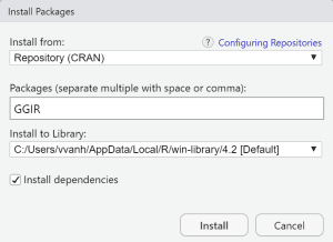
  1. In RStudio go to Toolbar -> Tools -> Install packages…
  2. Make sure the ‘Install from’ field is set to CRAN.
  3. Type GGIR in the empty field.
  4. Click install, the installation will automatically start. You may be prompted with questions, click yes.
  5. Note that an alternative route to installing R packages is with the command: install.package(“GGIR”, dependencies = TRUE), where you should replace “GGIR” by the package(s) you want to install.
10. Check R and GGIR version
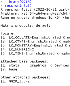
  1. Type library(GGIR) on the command line and press Enter.
  2. Type sessionInfo() on the command line and press Enter.
  3. This should show you in the console Window the R version, the GGIR version that is currently loaded, and various other information. In the example below you see that I had R version 4.2.2 and GGIR 2.8-2 installed at the time when I made the screenshot.

11. Some final notes on RStudio
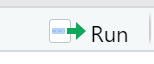
  1. Earlier in this blog post we asked you to use the Source button. It may be worth highlighting that there is another button next to the Source button, which is the Run button (see image). The Run button tells RStudio to only execute a specific script line or a selection of lines from the script. Next RStudio copies each of those lines to the console, runs them, and shows the output value. In theory you can also use the Run button and some GGIR users only use the GGIR button. However, there are couple of challenges with using the Run button: It can quickly clutter your console window with information you may not even be interested in, and it can easily lead to mistakes by forgetting to re-run parts of your script necessary for the computation. Therefore, the safest way to work with GGIR may be to use the Source button. In that way you know for sure that you always run all the lines in a script and that only information is printed to the console that is intended to be read by you.
  2. RStudio offers many shortkeys to do many of the operations fast. We encourage you to explore these as they can save you a lot of time. For example, Ctrl+A followed by Crtl+I tidies up the indentation of your script (Mac users will have to replace the Ctrl key by the Apple Command key).

Once you have mastered the above steps you should be all set to explore GGIR, either via the package vignette or via one of our GGIR training courses.

Why does GGIR facilitate the cut-points approach?

The ‘cut-points’ approach is one of the most criticized analytical approaches in the field of physical activity research. Despite the criticism, cut-points are still widely used. R package GGIR facilitates the use of cut-points and by that contributes to the continued use of cut-points. So, you may wonder: Why does GGIR facilitate such a controversial method? Do the people behind GGIR not know about the limitations of cut-points? To answer these questions, it may be good that I first explain what the ‘cut-points’ approach is.

What is the cut-points approach?

Wearable accelerometer data can be processed towards an indicator of body acceleration over time. Although acceleration is a meaningful kinematic indicator, researchers have not incorporated acceleration directly into physical activity guidelines. Instead, the research community prefers to phrase physical activity guidelines in terms of time spent in levels of energy expenditure. Levels of energy expenditure are defined based on a construct named Metabolic Equivalent of Task (MET).

There are various ways to calculate MET. The most common approach is to use Oxygen consumed in milliliters per minute per kilogram body mass divided by 3.5. To obtain the MET value for an activity type we divide this Oxygen value during the activity by the value in rest. As a final step we convert the MET values on a continuous scale to the categorical intensity levels named: sedentary, light, moderate, and vigorous. With thresholds typically chosen at 1.5, 3.0, and 6.0 MET.

Direct measurement of Oxygen consumption in the real life setting of study participants is not feasible. Therefore, other methods are used to estimate the MET levels. Accelerometry is one of those methods as it is feasible to implement under real life conditions. When using accelerometers, the cut-points are technically acceleration thresholds that attempt to segment the acceleration values into the before mentioned intensity levels. Cut-points are identified based on an optimisation procedure utilizing small studies involving the combined measurement of MET values with indirect calorimetry and acceleration with a wearable accelerometer.

Known criticism of the cut-point approach

  1. Cut-points assume that body acceleration differs by intensity (MET) level, which is not always true. Two activity types can have a different acceleration but the same intensity level, or come with the same acceleration while being in different intensity levels.
  2. Cut-points are derived from small sample size studies and by that not well representative for the wider population.
  3. Cut-points need to re-derived for each new accelerometer data processing approach, each age group, and each accelerometer attachment location.
  4. Cut-points collapse rich time series information into time spent in only three or four categories of behaviour.
  5. Cut-points may seem simple to implement but actually come with various non-trivial decisions. For example, epoch length, bout length, bout algorithm, and whether to allow for breaks in bouts.

As a side note – To some degree all these limitations also apply to machine learned models. But this blog post is about cut-points, I will save my thoughts about machine learning for a future blog post.

History of cut-points in GGIR

The cut-points approach was intentionally missing in the early versions of the code that would later become R package GGIR. I left them out because I hoped that that would help push the field away from cut-points. However, my somewhat idealistic ambition did not survive long. I abandoned it in 2012 when I was asked to design and implement the accelerometer data processing for the Pelotas birth cohorts in Brazil and the Whitehall study II in the United Kingdom. Especially the Pelotas birth cohort team was keen to have time spent in moderate or vigorous physical activity incorporated. Looking back, I had the following justifications to give in:

  • As an early career researcher I was keen to make an impact. Leading on the design of data processing pipeline would definitely be a nice boost to my experience. So, it seemed not worth the effort to make a big issue about including a widely used method like the cut-points method.
  • By letting the GGIR user choose their own cut-points, the responsibility for that choice lies with the user and not with me.
  • The cut-points approach can be interpreted as time spent in acceleration ranges. Therefore, I considered the debate around cut-points methods largely as an interpretation problem and not a methodological problem as such.

Nevertheless, a consequence of this decision is that GGIR users are confronted with the confusing reputation of cut-points as being both popular and widely criticised.

Why this blog post?

In this blog post I aim to share my personal views on the topic of MET level estimation with cut-points. I hope that by doing so I can provide some guidance to (new) GGIR users facing the confusing reputation of cut-points.

The problematic MET construct

To navigate the discussion around cut-points, I think it is important to first convince you that the MET construct itself is the main problem:

As you may have noticed the MET calculation comes with the assumption that dividing Oxygen consumption by body weight addresses variation in Oxygen consumption explained by body weight irrespective of the activity type being performed. However, it is well known in the field of exercise physiology that the relation between Oxygen consumption and body weight differs by activity type. For example, the classical textbook ‘Work Physiology’ by Åstrand and Rodahl already discussed this for VO2-max measurement. To truly normalise for body weight, we may need to divide by body weight to the power of X, where X differs per activity type. The problem of that, however, is that a different coefficient X for each activity type renders MET values incomparable across activity types. As a result, it is impossible to normalise Oxygen consumption for body weight across activity types.

Now you may say that the step in the MET calculation to divide by Oxygen consumption rest will address all this because it makes METs unit less. That would only be true if the over- or under correction for body weight in rest would be identical to the over-or under correction for body weight during each type of activity. As discussed above this is not what we would expect. Furthermore, if the direction of over- or under correction is reversed between rest and the activity type of interest then dividing by MET in rest will amplify the error.

Why is this a problem?

This is not a nuance. The inability to normalise for body weight invalidates MET as universal criterion method. It causes MET levels to be different between groups that differ in body weight despite performing exactly the same activity type, with bias that is activity type specific.

If you have access to measured MET values per activity type then you can see this for yourself by plotting the MET values from a single activity type as a function of body weight. In the activity type ‘sitting still’ you will probably see a negative slope, which indicates that MET overcorrects for body weight. As a result, it will push lighter individuals above the 1.5 MET cut-point towards light intensive activity. Similarly, you may see that MET also overcorrects for body weight causing heavier cycling individuals to be ranked as light active. In contrast, light individuals performing the same cycling activity could be classified as moderately active.

A second problem

A second problem with the MET construct based on Oxygen consumption is that it does not account for carbon dioxide production. As a result, it is a poor measure of energy expenditure when comparing groups that differ in diet. This is well known in exercise physiology and the reason why exercise physiologist typically try to standardise the diet of study participants prior to experiments. On a positive note, this second problem can partly be addressed by revising MET to incorporate both Oxygen and Carbon dioxide measurements.

Consequences

Any method developed to estimate MET values will struggle to remain valid when cross-validated in individuals with different body weight, different composition of activity types, and/or different diet. This is not because methods are inaccurate but a direct result of the MET construct itself.

Note that I am not discussing measurement errors in indirect calorimetry. It is the MET construct derived from the Oxygen data that is problematic, not the Oxygen data itself.

Also, it is important to note that the limitations of MET are not specific to cut-points but affect all attempts to estimate or classify MET levels, ranging from accelerometers, to heart rate sensors, to self-report methods, and from cut-point techniques to machine learning methods.

Biases in studies that evaluate cut-point methods

If you are somehow not convinced yet by my critiques on the MET construct then there is a second reason to be careful with studies that propose or evaluate methods to convert accelerometer data to MET values. Many of them come with one or both of the biases as listed below.

1. MET at epoch level unjustified

Energy metabolism can only be measured reliably during state aerobic energy metabolism. However, some studies incorrectly ignore this principle and assign the derived average MET level (during steady state) to each 5-60 second epoch within the steady state window. So, they assume that the MET level was constant during the steady state period. This is problematic because indirect calorimetry cannot provide evidence that the MET level is constant at such a high resolution.

Similarly, there have been studies who use the MET-compendium to assign MET values to epoch level data. This is equally problematic because those MET-compendium values were derived as average from steady state data and cannot be used as reference for epoch-level data. The epoch-level data represents the full within-individual variation in epoch-level energy expenditure, while the MET compendium only provides the average across a steady state window.

Both scenarios penalize accelerometer-based methods that are sensitive to true epoch-by-epoch variations in energy expenditure. Indirect calorimetry cannot capture this. Therefore, any study that evaluates a MET-classification method at a 1-minute or shorter epoch duration without proof of steady state energy metabolism for that epoch should be treated with high suspicion.

2. Inconsistencies in method implementation

The cut-points themselves are only one component of the cut-points method. The performance is also defined by other components such as:

    1. acceleration sensor version
    2. manufacturer software version and its configuration
    3. software to read and process the data
    4. efforts to monitor or correct for calibration error
    5. scripts to run the statistical analysis.

The implementation of cut-points methods often differs in more than only one of the components. For example, a common inconsistency across studies is the exact way MET in rest are derived. Using a different method for deriving MET in rest may cause a minor absolute bias, but could introduce a significant bias in the intensity levels that are extracted from it.

As a result, differences in performances across studies may then no longer be explained by the cut-points alone. This invalidates the comparison itself, the validation study is invalid. So, studies who do not pay attention to possible methodological differences should be treated with high suspicion.

Why then still facilitate cut-points in GGIR?

Despite all these limitations cut-points allow us to discriminate individuals with different behavioural time-use profiles. The estimates are interpretable as incremental levels of body acceleration. Body acceleration is known to be a kinematic characteristic of human behaviour. Further, it is proven to be a crude proxy for other physiological processes. The problem has been the interpretation of the method output as direct measure of those physiological processes. If we acknowledge that it is not true we actually create value.

Additionally, it may be important to point out that cut-points are not the only method GGIR facilitates. GGIR has also been used for:

  • deriving and comparing average acceleration during the entire day or during waking hours
  • deriving and comparing the distribution of acceleration values
  • preparing data for use with functional data analysis
  • deriving and comparing other behavioural metrics such as the intensity gradient and characterisation of the most active X hours per day

Next steps?

  1. Before investing more effort into MET classification we may first need to identify and internationally agree on a good measurement construct. Ideally, we need a measurement construct that is comparable across populations of different body weight and across activity types.
  2. It may be time to start expressing physical activity guidelines in terms of required acceleration levels. An advantage of such a guideline is that it can directly be incorporated into consumer wearables. Further, it avoids relying on the problematic MET construct. Especially when methods like cut-points are linear there is no added value of converting to MET, because both will explain the exact same variance in the data.
  3. More wide scale adoption of alternative analytical approaches. If needed, in parallel to the conventional methods such as cut-points. Reporting multiple outcomes in publications helps to build up reference values for those outcomes.

How to keep GGIR alive?

If we want Open-Source research software to remain functional and relevant then an ongoing maintenance effort is needed. At a basic level, the maintenance effort would include the preservation of functionality. For example, fixing major bugs and keeping the software up to date with changes in dependencies. At a more advanced level, the maintenance effort would also cover the improvement of existing functionality, adding new features, and providing support to users.

Software sustainability is a term closely related to software maintenance and refers to two aspects:

  • Designing software in a way that eases maintenance.
  • The strategy to enable software maintenance over time.

In this blog post I will focus on the second aspect in relation to Open-Source R package GGIR.

Sustainability models

As Open-Source software is free, we cannot use software sales to fund the maintenance effort. Therefore, I had to choose a different model. The model I chose is to maintain GGIR based on paid consultancies. It works as follows: GGIR users contract me to make specific enhancements to GGIR or to provide training on the use of GGIR. The experience and income I generate from doing these consultancies allow me to remain committed to the maintenance of GGIR. Although this has been and still is an effective model, it may be good to reflect on what other models I could use in addition to the consultancy service.

1. Individual sponsorship?

In an individual sponsorship the developer of the software would ask benefactors of the software to sponsor them. An example of this is the GitHub sponsorship model. This model offers two versions:

1a. Sponsorship as form of appreciation:

This sponsorship comes without any commitment from the developer. It is just a way for sponsors to demonstrate their appreciation for the developers’ ongoing efforts to maintain the Open-Source software.

At first, this approach feels tempting to adopt: It is easy to set-up and it reinforces the open science idea that the community sustains the software. However, I also see some problems with the individual sponsorship model:

  • Conflict with commercial activities: It could create the confusing impression that I am a charity. I am not sure how I would be able to keep a clear distinction between what I do as a paid consultant and what activities could reflect the sponsorship donations.
  • Income insufficient: It is hard to imagine that this form of sponsorship can generate sufficient income to live from.
  • Unfair in relation to co-contributors: Sponsorships typically go to well-known developers and less prolific or more junior contributors may then miss out.

1b. Sponsorship as a service:

In this sponsorship type the sponsor expects a specific commitment from the developer. For example, to be available for a call once per month or to give higher priority to the needs of a sponsor. Sometimes this is done in the form a retainer agreement. The challenges I foresee here are:

  • Users may not need long term support: Once the client knows their way around GGIR the need for support will reduce, while the need for maintenance efforts continues. As a result, the service will effectively turn into the before mentioned ‘sponsorship as a form of appreciation’.
  • Hard to define a standard service description: Some GGIR users may only need minor support, while others GGIR user require substantial time investments. This makes it difficult to come up with a standard service model. Asking for €1000 per year would seem expensive for the first group but cheap for the second group.

2. Project-based sponsorship?

Examples of sponsorship at project level are the sponsorships provided by NumFocus and CZI. Project-based sponsorship makes it easier to share sponsorship income across developers compared with the individual sponsorship as discussed above. Further, if I would register as a foundation, which some of these sponsors require, it would become easier to separate project-based sponsorship from commercial activities. Nonetheless, for GGIR a project-based sponsorship may not be the most intuitive approach:

  • Sponsorships typically designed for teams: It appears that most sponsorships are designed to help teams-based organisations, while in the case of GGIR maintenance is primarily done by me alone. Of course, I could start assembling a team, but in the initial phase all the administrative and coordination burden will be on me.
  • Limited amount of funding opportunities: Both NumFocus and CZI are based in the United States. I am not aware of any European sponsorships for Open Source software that I am eligible for. Most opportunities seem to be restricted to academic researchers only.

Project-based sponsorships are potentially valuable but are best led by an academic researcher familiar with grant applications.

3. Linking Open-Source software to commercial products and services?

At the moment I have no plans in this direction, but in theory I could offer the following services:

  • Cloud service to provide data analysis.
  • Exclusive faster second version of GGIR that can only be used with a specific accelerometer brand.

A part of the revenue generated from these services could then be used for maintenance of the software. My feeling for now is that both ideas require a level of expertise that I do not have.

4. Advertisements?

Incorporating advertisements in software is common with mobile phone apps. In the case of GGIR, I already make subtle advertisement for my consultancy services as Accelting. If I wanted to get external advertisers, then I am not sure who would be a good candidate advertiser. The strength of GGIR is that it works across accelerometer brands, so allowing accelerometer manufacturers to advertise their product inside GGIR does not seem fitting. However, other forms of advertising may work fine. Interested? I am happy to have a chat.

Conclusion

The best route forward seems keeping the focus on my paid consultancy for the following reasons:

  • A clear commitment between me, doing the work, and the client paying me.
  • Paying clients ensure that all maintenance efforts are tailored to the most urgent needs of the user community.
  • It counters the idea that Open-Source software is inherently unsustainable and should be supported like we support charities. By doing business based on Open-Source software I demonstrate the value and sustainability of GGIR as Open-Source software.

That said, this shouldn’t stop anyone else from contributing to GGIR in complementary ways.

How you can contribute?

  • Are you in a position to apply for funding to help improve GGIR? If yes, please do so, and I’d be more than happy to collaborate and support you where needed.
  • Do you have software development skills and are you in a position to help contribute to GGIR then, again, please do so. Being part of the open source software community is rewarding in itself!
  • If you know of any other sustainability model not listed here then let me know.


How to measure PA guideline adherence?

I often get asked the question: How can we quantify a person’s adherence to the physical activity (PA) guidelines with an accelerometer? In this blog post I will try to answer that question.

How we arrived here

As you may know, there are many ways to process accelerometer data towards an estimate of a person’s physical activity. Also, a decision needs to be made on what accelerometer to use and where to place it on the body. An accelerometer-based research method is the combination of sensor type, attachment location, algorithms used, and the software implementation of those algorithms. There is no universally agreed method for physical activity assessment, by which a variety of methods have been used across the physical activity research literature. PA guidelines have been constructed based on the evidence provided by this literature.

PA guideline reports usually do not guide us on what method we should use to measure adherence to the guideline. This is understandable: The underlying evidence does not use a consistent method, which makes it hard to provide such guidance. The resulting confusion about how guideline adherence should be quantified leads many people in this research field to wonder: What method should I use?

Why there is no simple answer

Before I continue, I would like to point out that a measurement method determines the definition of what is being measured. Publications sometimes start with an elegant definition of physical activity, but it is the measurement method that defines what physical activity is, not the researcher. The researcher only chooses the method.

This effectively means that the definition of physical activity according to the PA guidelines is a weighted average of all the methods that underlie the PA guidelines. Consequently, we can only quantify adherence to the PA guidelines if we apply the same weighted average of methods to our study participants. To me this seems infeasible as you would have to instruct your study participant to wear accelerometers from a variety of brands on multiple body locations simultaneously. Note that I am not even discussing self-report methods for physical activity, which would further complicate this effort.

Therefore, monitoring adherence to PA guidelines is not straightforward. Any attempt to measure guideline adherence will result in a biased estimate relative to the multi-method evidence on which a guideline is based. We should not blame methods for not being comparable, we should blame ourselves as a research community for having an ambiguous definition of physical activity by which it is impossible for any method to comply with it.

Surely a more accurate method is what we need?

Now imagine that we had access to a super method able to measure people’s energy expenditure, count their steps, and detect activity types without any error and with the highest level of feasibility. Even such a super method would be unsuitable for evaluating adherence to the current PA guidelines, for the simple reason that this super method was never used to develop the PA guidelines in the first place. Instead, we would need a method that replicates the pooled imperfections of the methods that underlie the current PA guidelines. As I mentioned before, this would be an impossible task.

Looking for a solution

I am keen to help the community to find a solution. If only, it was to avoid having to justify all the time why we cannot accurately quantify PA guideline adherence. I already started drafting a short communication for a journal with colleagues. Well, for now it is a good exercise in trying to shape our thoughts, even if we decide not to submit it in the end.

In the meantime, I think it is important to make people aware that this is a complex challenge, which should not be treated as just a methodological problem, just a harmonisation problem, just a research communication problem, or just a PA guideline construction problem. We may even need to rethink the whole research ecosystem to address the actual issue. Here, we may benefit from looking for inspiration in other professional fields that produce public health guidelines. If you have thoughts on this then I would love to hear from you.

High frequencies in an acceleration signal

It is often argued that high frequency components in an acceleration signal should be omitted. The motivation given is that these high frequencies are a consequence of machine noise or vibrations, or at least not human. With this comes the assumption that human movement can only cause low frequency components. Here, the division line between low- and high frequencies varies across studies from 5 to 20 Hertz.

Intermezzo – What do we mean by ‘frequencies in an acceleration signal’?

Joseph Fourier showed that a time series can be described as the combination of multiple sine waves, each with their own frequency characteristic. A periodogram is a visualisation of the contribution of all those sines to the total variance in a time series. The frequencies are shown on the horizontal axis and their contribution to the variance is displayed on the vertical axis.

Are high frequencies truly just noise?

At first, the idea that high frequencies are not caused by human movement sounds plausible: A washing machine at top speed rotates at around 23 Hertz. Surely our body would not be capable of producing that kind of rotations.

Nevertheless, very little empirical research has been done to support the idea that all high frequencies are redundant. To me it does not feel satisfying to embrace this widespread belief without having clear evidence for it. For example, it would be helpful to know the relative contribution of human movement, machine noise, and non-human vibrations to the frequency content of a signal. Also, it would be good to know whether these contributions vary across the frequency spectrum. Such insights would help to make an informed decision on what frequency filter to use, if any.

To gain a better understanding I did the following short experiments together with my project partners in Regensburg:

Accelerometer data from walking and non-wear

The acceleration signal was collected with a hip-worn accelerometer in walking. This tri-axial accelerometer was configured to collect data at 100 Hertz. Additionally, I have a recording of that same accelerometer when it was lying still on a table (not worn). Both signals have a length of 45 seconds and I only look at the vertical (longitudinal) signal. The periodograms show that the frequency density is consistently higher for walking than when the accelerometer is not worn. Not just during the low frequencies below 10 Hertz, but all the way up to 50 Hertz. This indicates that the high frequencies in the signal for walking are not simply explained by a natural level of noise seen when the sensor is not worn.

Enhancing theoretical understanding with artificial data

I complemented these accelerometer experiments with an artificial signal. The artificial signal is a rectified 1 Hertz sine wave, which looks like a pendulum motion. Pendulum motions are often used as a model for human movement where smooth rotations are interrupted by abrupt changes in movement direction. Next, I sum this artificial signal with the experimental non-wear data (discussed above). The resulting periodogram shows not only a peak for the resulting 2 Hertz frequency of the pendulum, but also it’s harmonics at higher frequencies. Harmonics are a natural consequence of waves that do not have a perfect sine shape. In sound, the specific shape of the wave is what gives our voice and musical instruments their characteristic sound. In acceleration signals the harmonics give the wave it’s movement specific shape.

Interpretation

The periodogram of the artificial signal looks suspiciously similar to what we see in the periodogram of the signal for walking. The peaks in both have a gradual decline towards the top frequency.

Based on this it would seem likely that higher frequencies in an acceleration signal are not only caused by machine noise but also by the harmonics of movement. In fact, the contribution of the harmonics is much larger than the contribution of signal noise in this little experiment. Further, the experiment shows that even a simple 2 Hertz pendulum movement can produce high frequency components. However, it is not a single human body joint that is rotating at these high frequencies. It is the combined impact of multiple joint movements and the interaction of the human body segments with each other and with the environment (floor in this case) that causes the pendulum shape. The pendulum shape in turn produces a broad frequency profile. If we would filter out these harmonics in the signal, we would lose the detailed representation of body movement in the original signal.

How about sensor vibrations?

The other explanation offered for high frequencies is that they represent vibrations of the accelerometer relative to the human body. For example, as a result of loose attachment with an elastic strap or because of skin movement relative to the underlying bones. In general, when objects vibrate they tend to vibrate at their, so called, eigenfrequency. However, when we look at the periodogram of walking we see a homogeneous increase in density of all frequencies. If the high frequencies would only be caused by a vibrations then we would expect to see an increase near the eigenfrequency or a set of eigenfrequencies for those vibrations.

Conclusion

In conclusion, high frequencies in an acceleration signal can represent body movement. Therefore, filtering out high frequencies may not necessarily be a good thing. Not filtering the signal will preserve the detailed representation of the movement. Additional advantages of not filtering are that it is computationally faster, and that signal processing is potentially easier to reproduce as there are less computational steps.

In the specific use case of assessing human daily physical activity I recommend the following:

  • Do not filter out the high frequencies unless there is clear evidence that filtering gives better estimates of physical activity. To my knowledge there are no studies that show the added value of filtering.
  • Only consider filtering out high frequencies if data comparability between accelerometer brands/generations is critical to your research question. Accelerometer brands and generations can have different sensitivities to human body acceleration. By filtering out high frequencies you create a less precise but potentially more comparable acceleration signal.

The exploration described in this blog post is part of the project I am doing for the University of Regensburg, Germany.